renv::install("ggpubr")Exercise - Block 4
Learning Objectives
Upon completing this exercise block, you will be able to:
- Add statistical summaries and regression lines to
ggplot2plots usinggeom_smooth(). - Incorporate correlation coefficients and p-values into plots using functions from the
ggpubrpackage. - Compare groups and display statistical test results (e.g., t-test p-values) on boxplots.
- Create informative volcano plots to visualize differential expression data.
- Label specific points on plots using
ggrepelto avoid overplotting.
Introduction to Statistical Annotations
In this block, we will delve into enhancing our ggplot2 visualizations with statistical summaries and annotations. This is crucial for presenting data analysis results effectively and making plots more informative. We will explore how to add regression lines and their confidence intervals using geom_smooth(), incorporate correlation coefficients and p-values with the ggpubr package, and create specialized plots like volcano plots. Furthermore, we will learn to use ggrepel for intelligent labeling of data points, ensuring readability even with many labels.
Installing packages
Packages
library(ggplot2)
library(ggpubr)
library(dplyr)
Exploratory data analysis
data <- readRDS(gzcon(url(
  "https://raw.githubusercontent.com/urppeia/publication_figs/main/data.rds"
)))

rownames(data$counts) <- data$counts$Gene_ID
data$counts <- data$counts[, -1]
Exercise 1: Scatter plot with regression line
Let’s investigate the relationship between the log-fold change (LFC) at 3h and 24h. Understanding this correlation can reveal how gene expression changes evolve over time. We will use geom_smooth() to visualize this relationship with a linear regression line and its confidence interval, providing insight into the trend and variability.
A. Create a scatter plot of sucrose_3h_lfc vs. sucrose_24h_lfc from the data$diff dataframe.
B. Add a linear regression line and confidence interval to the plot.
Solution
p1 <- ggplot(data$diff, aes(x = sucrose_3h_lfc, y = sucrose_24h_lfc)) +
  geom_point() +
  labs(
    title = "LFC Correlation: 3h vs. 24h",
    x = "LFC at 3h",
    y = "LFC at 24h"
  ) +
  theme_bw() # Apply black and white theme for cleaner look
p1 + geom_smooth(method = "lm")
`geom_smooth()` using formula = 'y ~ x'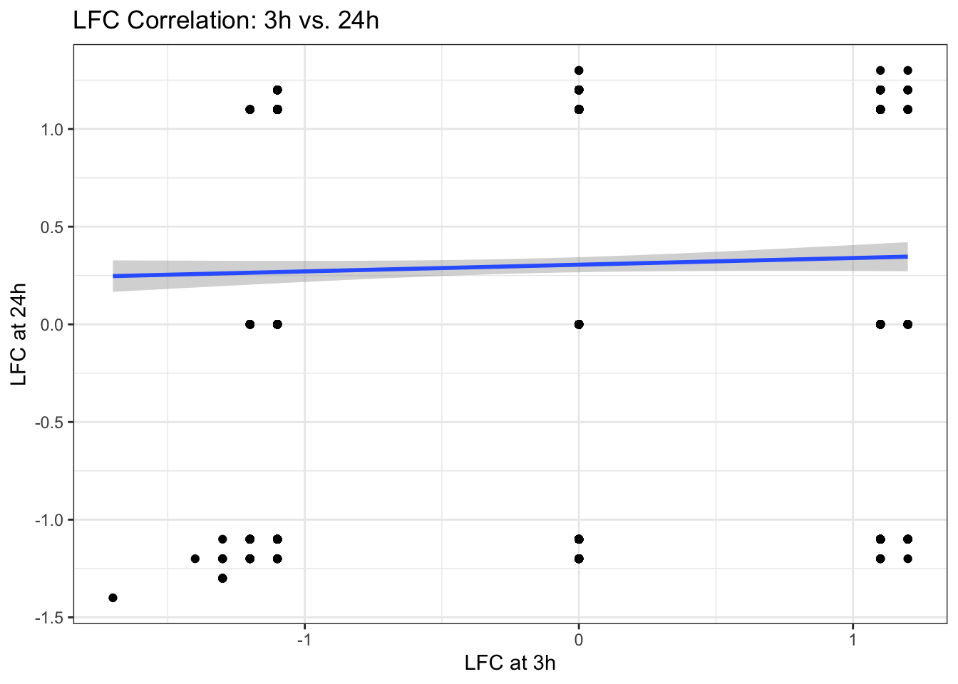
Exercise 2: Adding correlation coefficient
Now, let’s add the Pearson correlation coefficient and p-value to the plot from Exercise 1. The stat_cor() function from the ggpubr package is particularly useful for this, as it automatically calculates and displays these statistical metrics directly on the plot, providing a quantitative measure of the relationship.
A. Use stat_cor() from the ggpubr package to add the correlation.
Solution
p2 <- p1 + stat_cor(method = "pearson") + theme_bw() # Apply black and white theme
p2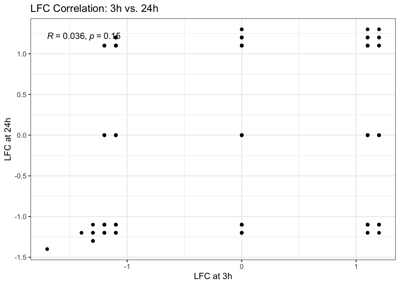
Exercise 3: Boxplot with p-values
Let’s compare the expression of a single gene between the “none” and “sucrose” conditions at 24h. Boxplots are excellent for visualizing the distribution of expression levels across different conditions. Gene expression data is often log-transformed to better visualize the variance and make the distribution more symmetric. We will use a log2(expression + 1) transformation.
To statistically compare these groups, we will use stat_compare_means() from ggpubr, which can perform various statistical tests (e.g., t-test) and display the resulting p-values directly on the plot.
A. First, prepare the data. Choose a gene that is significantly differentially expressed at 24h.
B. Create a boxplot of the log2 transformed expression for the selected gene, comparing “none” and “sucrose” conditions.
C. Add the p-value from a t-test comparing the two groups. Use stat_compare_means().
Solution
# Find a significant gene at 24h
sig_gene_24h <- data$diff[data$diff$sucrose_24h_pval < 0.05 & abs(data$diff$sucrose_24h_lfc) > 1, ][1, "Gene_ID"]

# Prepare the data for plotting
plot_data <- data.frame(
  expression = as.numeric(data$counts[sig_gene_24h, ]),
  compound = data$anno$compound,
  time = data$anno$time
) %>%
  filter(time == "24 hour")

# Create the plot
p3 <- ggplot(plot_data, aes(x = compound, y = log2(expression + 1), fill = compound)) +
  geom_boxplot() +
  labs(
    title = paste("Expression of gene", sig_gene_24h, "at 24h"),
    x = "Compound",
    y = expression("Log"[2] * " Expression Levels")
  ) +
  theme_bw() # Apply black and white theme

# Add the p-value
p3 + stat_compare_means(method = "t.test")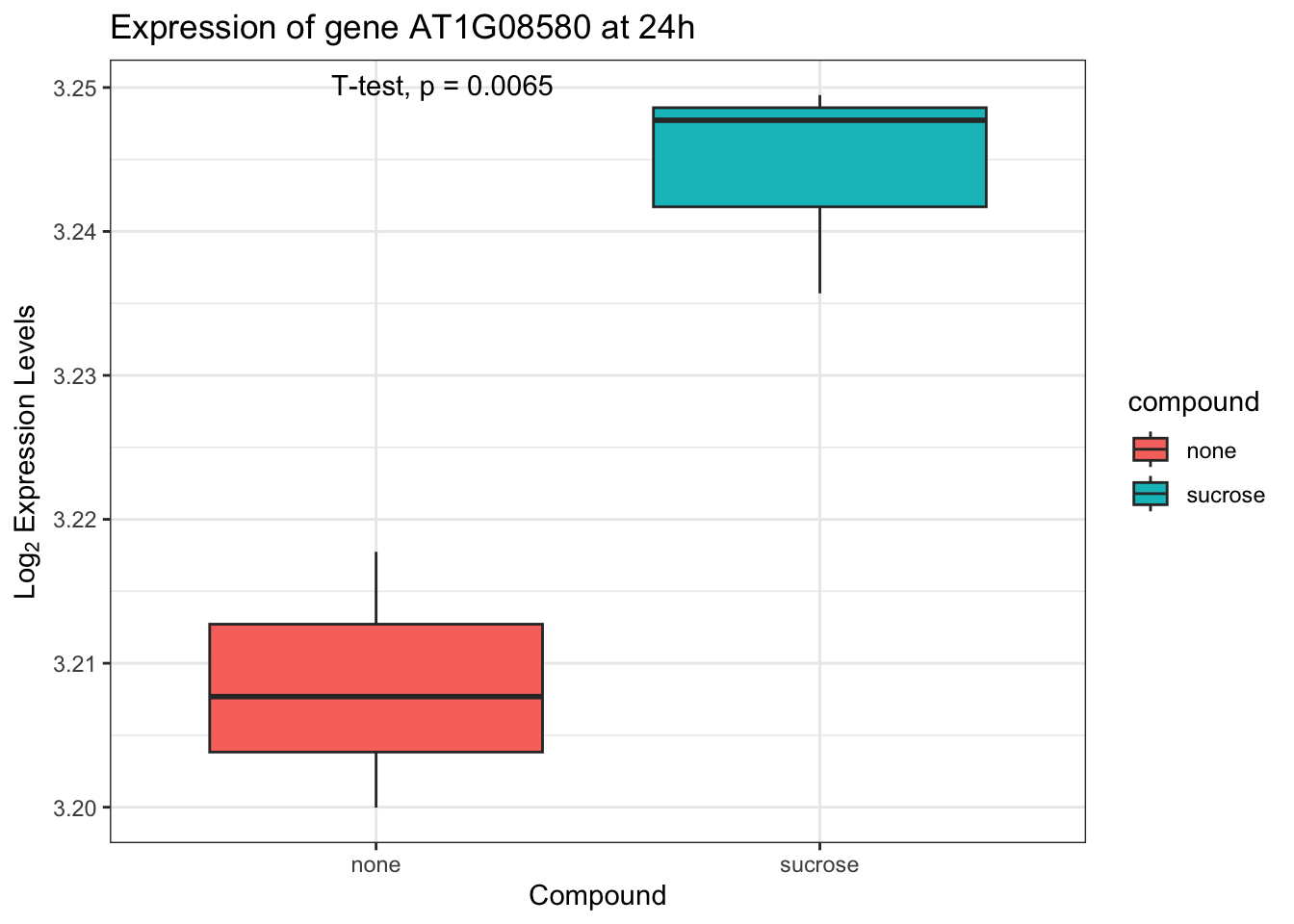
Exercise 4: Volcano plot
Let’s create a volcano plot to visualize the differential expression results at 24h. A volcano plot is a powerful visualization that combines information about fold-change (on the x-axis) and statistical significance (on the y-axis). By plotting -log10(p-value), we can easily spot the most statistically significant genes, as smaller p-values will correspond to larger values on the y-axis. This allows us to quickly identify genes that are both substantially and statistically differentially expressed. We will also use ggrepel::geom_text_repel() to add labels to significant genes without overlapping, ensuring readability.
A. Create a scatter plot of sucrose_24h_lfc vs. -log10(sucrose_24h_pval).
B. Color the points based on significance. For example, use red for genes with sucrose_24h_pval < 0.05 and abs(sucrose_24h_lfc) > 1.
C. Add labels to the significant genes.
Solution
# Add a column to indicate significance
data$diff$significant <- ifelse(data$diff$sucrose_24h_pval < 0.05 & abs(data$diff$sucrose_24h_lfc) > 1, "yes", "no")

# Create the volcano plot
p4 <- ggplot(data$diff, aes(x = sucrose_24h_lfc, y = -log10(sucrose_24h_pval), color = significant)) +
  geom_point(alpha = 0.5) +
  scale_color_manual(values = c("yes" = "red", "no" = "grey")) +
  labs(
    title = "Volcano Plot at 24h",
    x = "Log2 Fold Change",
    y = expression("-Log"[10] * " (" * italic(p) * "-value)")
  ) +
  theme(legend.position = "none") +
  theme_bw() # Apply black and white theme

# Add labels to significant genes
p4 + ggrepel::geom_text_repel(
  data = subset(data$diff, significant == "yes"),
  aes(label = Gene_ID),
  size = 3,
  box.padding = 0.5
)
Warning: ggrepel: 63 unlabeled data points (too many overlaps). Consider
increasing max.overlaps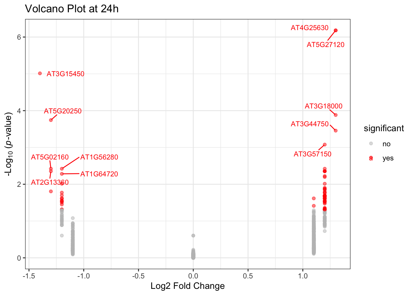
Exercise 5: Correlation of two genes
Another common task is to investigate the correlation between the expression of two specific genes. This can reveal co-regulation or related functions. Log-transforming the expression data can make the relationship between genes more linear and easier to interpret, especially with a wide dynamic range. Let’s dynamically select the top 2 most expressed genes for this exercise.
A. Find the top 2 most expressed genes in the data$counts dataframe.
B. Create a scatter plot of the log2 transformed expression of these two genes.
C. Add a regression line and the Pearson correlation coefficient to the plot.
Solution
# Find the top 2 most expressed genes
gene_means <- rowMeans(data$counts, na.rm = TRUE)
top_genes <- names(sort(gene_means, decreasing = TRUE)[1:2])
gene1 <- top_genes[1]
gene2 <- top_genes[2]

# Prepare the data for plotting
plot_data_corr <- data.frame(
  gene1_expr = as.numeric(data$counts[gene1, ]),
  gene2_expr = as.numeric(data$counts[gene2, ]),
  compound = data$anno$compound,
  time = data$anno$time
)

# Remove rows with NA values
plot_data_corr <- na.omit(plot_data_corr)

# Create the scatter plot
p5 <- ggplot(plot_data_corr, aes(x = log2(gene1_expr + 1), y = log2(gene2_expr + 1))) +
  geom_point(aes(color = compound, shape = time)) +
  geom_smooth(method = "lm", formula = "y ~ x") +
  stat_cor(method = "pearson") +
  labs(
    title = paste("Correlation between", gene1, "and", gene2),
    x = expression("Log"[2] * " Expression Levels"),
    y = expression("Log"[2] * " Expression Levels")
  ) +
  theme_bw()
p5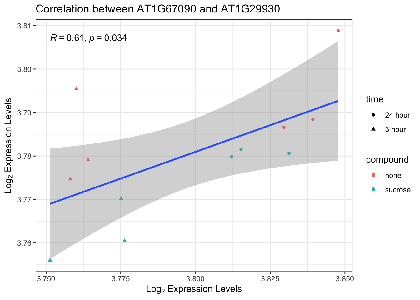
Session information
Tip
sessionInfo()R version 4.5.1 (2025-06-13)
Platform: aarch64-apple-darwin20
Running under: macOS Tahoe 26.0.1
Matrix products: default
BLAS: /Library/Frameworks/R.framework/Versions/4.5-arm64/Resources/lib/libRblas.0.dylib
LAPACK: /Library/Frameworks/R.framework/Versions/4.5-arm64/Resources/lib/libRlapack.dylib; LAPACK version 3.12.1
locale:
[1] en_US.UTF-8/en_US.UTF-8/en_US.UTF-8/C/en_US.UTF-8/en_US.UTF-8
time zone: Europe/Zurich
tzcode source: internal
attached base packages:
[1] stats graphics grDevices datasets utils methods base
other attached packages:
[1] dplyr_1.1.4 ggpubr_0.6.2 ggplot2_4.0.0
loaded via a namespace (and not attached):
[1] Matrix_1.7-3 gtable_0.3.6 jsonlite_2.0.0
[4] compiler_4.5.1 BiocManager_1.30.26 ggsignif_0.6.4
[7] renv_1.1.5 Rcpp_1.1.0 tidyselect_1.2.1
[10] tidyr_1.3.1 splines_4.5.1 scales_1.4.0
[13] yaml_2.3.10 fastmap_1.2.0 lattice_0.22-7
[16] R6_2.6.1 labeling_0.4.3 generics_0.1.4
[19] Formula_1.2-5 knitr_1.50 backports_1.5.0
[22] htmlwidgets_1.6.4 ggrepel_0.9.6 tibble_3.3.0
[25] car_3.1-3 pillar_1.11.1 RColorBrewer_1.1-3
[28] rlang_1.1.6 broom_1.0.10 xfun_0.53
[31] S7_0.2.0 cli_3.6.5 mgcv_1.9-3
[34] withr_3.0.2 magrittr_2.0.4 digest_0.6.37
[37] grid_4.5.1 nlme_3.1-168 lifecycle_1.0.4
[40] vctrs_0.6.5 rstatix_0.7.3 evaluate_1.0.5
[43] glue_1.8.0 farver_2.1.2 abind_1.4-8
[46] carData_3.0-5 rmarkdown_2.30 purrr_1.1.0
[49] tools_4.5.1 pkgconfig_2.0.3 htmltools_0.5.8.1