Exercise - Block 1

Data for the course

data <- readRDS(gzcon(url(
  "https://raw.githubusercontent.com/urppeia/publication_figs/main/data.rds"
)))

str(data)

List of 3
 $ counts:'data.frame': 1642 obs. of  13 variables:
  ..$ Gene_ID   : chr [1:1642] "AT1G01090" "AT1G01100" "AT1G01300" "AT1G01320" ...
  ..$ ERR1736192: num [1:1642] 8.95 10.71 8.26 10.47 9.6 ...
  ..$ ERR1736193: num [1:1642] 8.75 11.05 8.62 9.85 9.74 ...
  ..$ ERR1736194: num [1:1642] 8.94 10.76 8.32 10.55 9.43 ...
  ..$ ERR1736195: num [1:1642] 8.8 10.93 8.52 10.17 9.66 ...
  ..$ ERR1736196: num [1:1642] 8.88 10.59 8.35 10.64 9.49 ...
  ..$ ERR1736197: num [1:1642] 8.78 11.02 8.49 9.91 9.76 ...
  ..$ ERR1736198: num [1:1642] 8.92 10.72 8.33 10.46 9.5 ...
  ..$ ERR1736199: num [1:1642] 8.92 11 8.73 9.84 9.85 ...
  ..$ ERR1736200: num [1:1642] 8.86 10.7 8.25 10.54 9.48 ...
  ..$ ERR1736201: num [1:1642] 8.88 11.04 8.44 9.75 9.78 ...
  ..$ ERR1736202: num [1:1642] 8.93 10.6 8.32 10.63 9.43 ...
  ..$ ERR1736203: num [1:1642] 8.81 10.99 8.34 10 9.61 ...
 $ diff  :'data.frame': 1642 obs. of  6 variables:
  ..$ Gene_ID         : chr [1:1642] "AT1G01090" "AT1G01100" "AT1G01300" "AT1G01320" ...
  ..$ Gene_name       : chr [1:1642] "PDH-E1 ALPHA" "RPP1A" "APF2" "" ...
  ..$ sucrose_24h_pval: num [1:1642] 0.591 0.569 0.565 0.743 0.884 ...
  ..$ sucrose_24h_lfc : num [1:1642] 1.1 1.1 1.1 0 0 0 0 1.1 0 1.1 ...
  ..$ sucrose_3h_pval : num [1:1642] 0.998 0.998 0.998 0.998 0.998 ...
  ..$ sucrose_3h_lfc  : num [1:1642] 0 -1.1 0 1.1 -1.1 0 1.1 0 0 1.1 ...
 $ anno  :'data.frame': 12 obs. of  4 variables:
  ..$ Sample_ID: chr [1:12] "ERR1736192" "ERR1736193" "ERR1736194" "ERR1736195" ...
  ..$ compound : chr [1:12] "none" "none" "sucrose" "sucrose" ...
  ..$ dose     : chr [1:12] "none" "none" "15 millimolar" "15 millimolar" ...
  ..$ time     : chr [1:12] "24 hour" "3 hour" "24 hour" "3 hour" ...

data$anno

    Sample_ID compound          dose    time
1  ERR1736192     none          none 24 hour
2  ERR1736193     none          none  3 hour
3  ERR1736194  sucrose 15 millimolar 24 hour
4  ERR1736195  sucrose 15 millimolar  3 hour
5  ERR1736196     none          none 24 hour
6  ERR1736197     none          none  3 hour
7  ERR1736198  sucrose 15 millimolar 24 hour
8  ERR1736199  sucrose 15 millimolar  3 hour
9  ERR1736200     none          none 24 hour
10 ERR1736201     none          none  3 hour
11 ERR1736202  sucrose 15 millimolar 24 hour
12 ERR1736203  sucrose 15 millimolar  3 hour

Overview of the Dataset

This RNA-seq dataset (GEO: GSE102374, SRA: PRJNA397585) comes from the tomato plant (Solanum lycopersicum). The experiment investigates how sucrose treatment affects gene expression in tomato over time. Each sequencing run (ERR1736192–ERR1736203) corresponds to one biological replicate under a specific treatment and timepoint.

Biological Context

Sucrose is not only a carbon source but also acts as a signaling molecule in plants, influencing growth, metabolism, and stress responses. By comparing gene expression profiles after sucrose exposure at 3 h and 24 h, the study aims to identify genes involved in early sugar signaling and longer-term metabolic regulation in tomato.

Experimental Design

Condition	Compound	Dose	Timepoint	Replicates (ERR IDs)
Control	none	none	3 h	ERR1736193, ERR1736197, ERR1736201
Control	none	none	24 h	ERR1736192, ERR1736196, ERR1736200
Sucrose-treated	sucrose	15 mM	3 h	ERR1736195, ERR1736199, ERR1736203
Sucrose-treated	sucrose	15 mM	24 h	ERR1736194, ERR1736198, ERR1736202

Total samples: 12
Design: 2 × 2 factorial (Treatment × Time)
Replicates: 3 per condition

Experimental Aim

To characterize transcriptional changes in tomato induced by sucrose at early (3 h) and later (24 h) timepoints, revealing genes and pathways regulated by sugar signaling.

Summary

This is a plant RNA-seq time-course experiment from Solanum lycopersicum, testing sucrose signaling effects. It illustrates a balanced factorial design, ideal for learning how to:

Interpret replicates and contrasts,
Model treatment × time interactions
Perform biological interpretation

Exploratory data analysis

Check the number of samples and genes in these data

head(data$counts)

    Gene_ID ERR1736192 ERR1736193 ERR1736194 ERR1736195 ERR1736196 ERR1736197
1 AT1G01090   8.951818   8.745436   8.936055   8.796355   8.881562   8.783848
2 AT1G01100  10.714686  11.049205  10.760942  10.925465  10.586018  11.018331
3 AT1G01300   8.262611   8.621839   8.317833   8.524731   8.351529   8.490846
4 AT1G01320  10.474282   9.846080  10.547565  10.166405  10.638864   9.910971
5 AT1G01620   9.602057   9.741940   9.433688   9.660392   9.487521   9.759061
6 AT1G01960   7.992299   8.164980   7.940793   8.188539   8.066384   8.091465
  ERR1736198 ERR1736199 ERR1736200 ERR1736201 ERR1736202 ERR1736203
1   8.918614   8.917665   8.859714   8.880689   8.925662   8.810786
2  10.720866  11.003460  10.697236  11.038316  10.602965  10.990252
3   8.326726   8.726843   8.252066   8.438347   8.321741   8.337898
4  10.459285   9.842758  10.536018   9.752592  10.629175  10.004448
5   9.495713   9.854984   9.475491   9.780328   9.425490   9.608561
6   7.887148   8.068782   8.022251   7.938457   7.981151   8.096472

The first column contains gene IDs. We can replace put them as row names, and remove the character column

rownames(data$counts) <- data$counts$Gene_ID
data$counts <- data$counts[,-1]

head(data$counts)

          ERR1736192 ERR1736193 ERR1736194 ERR1736195 ERR1736196 ERR1736197
AT1G01090   8.951818   8.745436   8.936055   8.796355   8.881562   8.783848
AT1G01100  10.714686  11.049205  10.760942  10.925465  10.586018  11.018331
AT1G01300   8.262611   8.621839   8.317833   8.524731   8.351529   8.490846
AT1G01320  10.474282   9.846080  10.547565  10.166405  10.638864   9.910971
AT1G01620   9.602057   9.741940   9.433688   9.660392   9.487521   9.759061
AT1G01960   7.992299   8.164980   7.940793   8.188539   8.066384   8.091465
          ERR1736198 ERR1736199 ERR1736200 ERR1736201 ERR1736202 ERR1736203
AT1G01090   8.918614   8.917665   8.859714   8.880689   8.925662   8.810786
AT1G01100  10.720866  11.003460  10.697236  11.038316  10.602965  10.990252
AT1G01300   8.326726   8.726843   8.252066   8.438347   8.321741   8.337898
AT1G01320  10.459285   9.842758  10.536018   9.752592  10.629175  10.004448
AT1G01620   9.495713   9.854984   9.475491   9.780328   9.425490   9.608561
AT1G01960   7.887148   8.068782   8.022251   7.938457   7.981151   8.096472

dim(data$counts)

[1] 1642   12

Check if the data is normalized

boxplot(data$counts)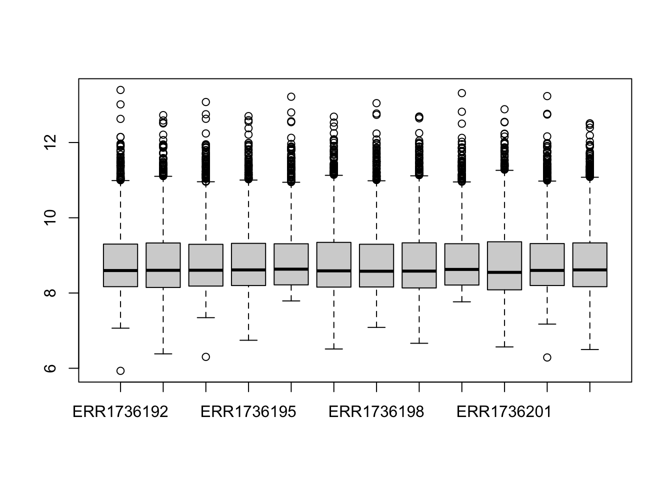

Exercise 1

A. Sample names are not properly readable. Rotate them to make perpendicular to the x-axis.

Tip

boxplot(data$counts, las = 2)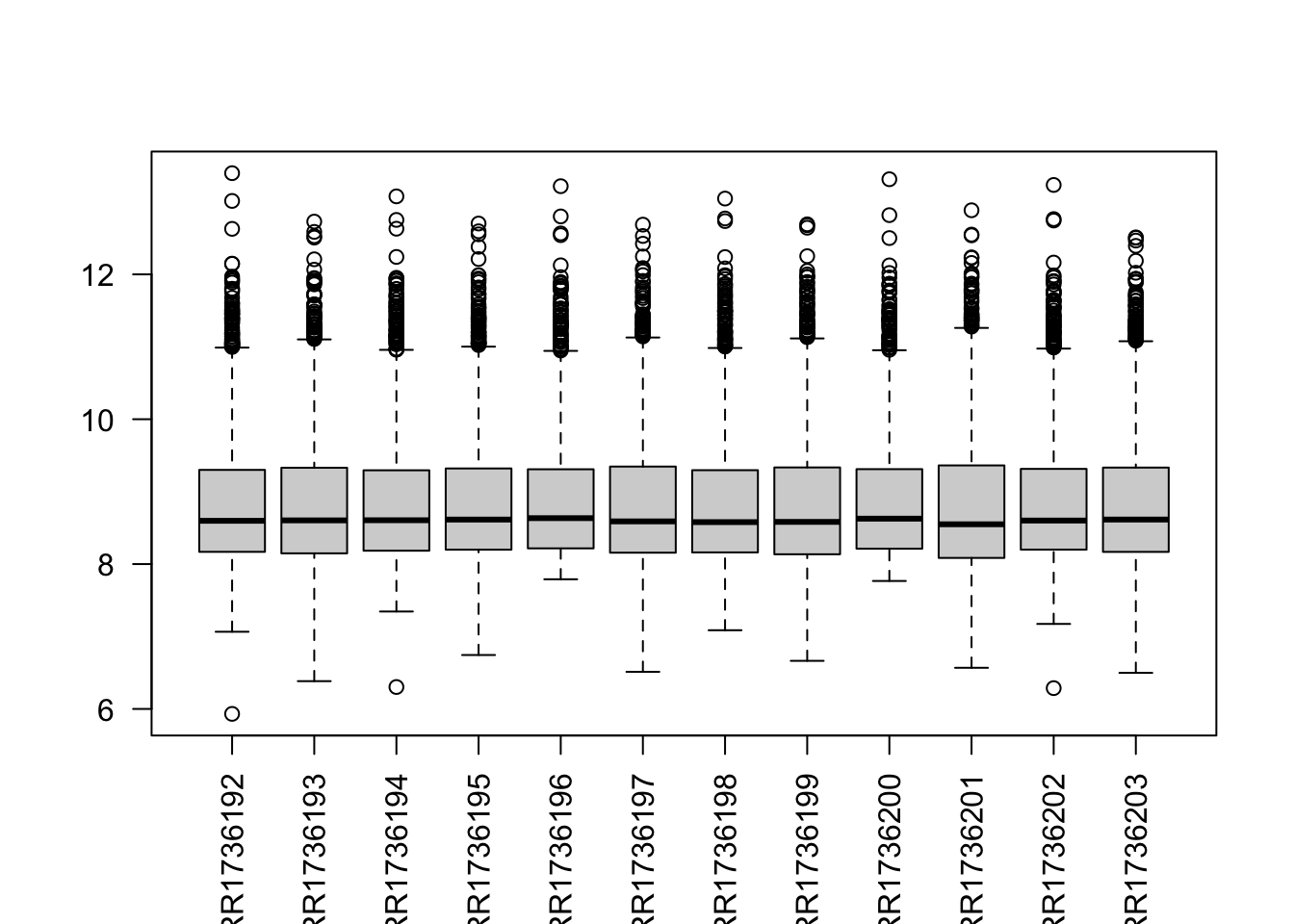

B. Remove the boxplot outliers

Tip

boxplot(data$counts, las = 2, outline = FALSE)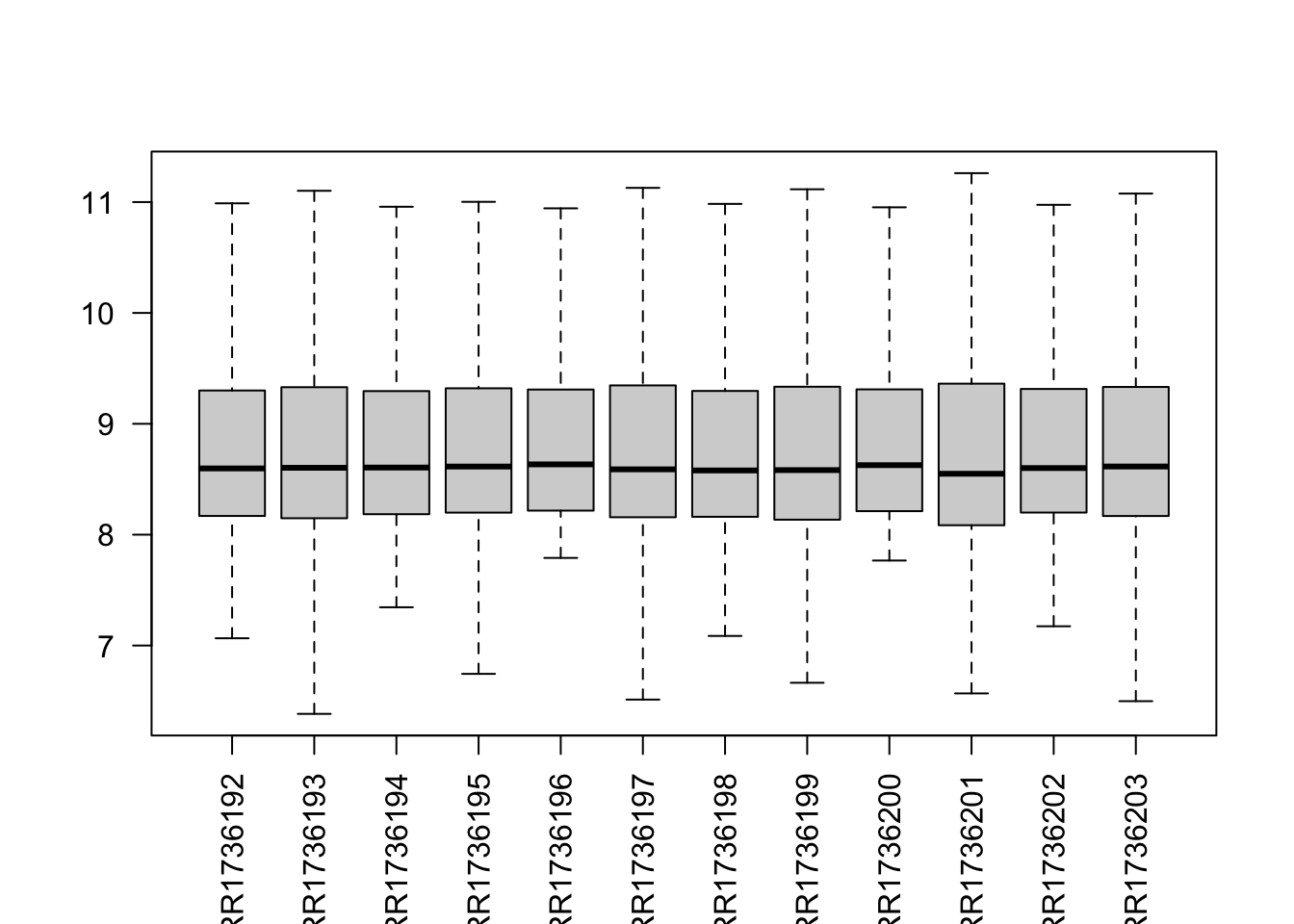

Mean expression per sample

sample_means <- colMeans(data$counts)

barplot(sample_means, las = 2, col = "skyblue",
        border = "gray40",
        main = "Mean normalized expression per sample",
        ylab = "Mean expression",
        cex.names = 0.8)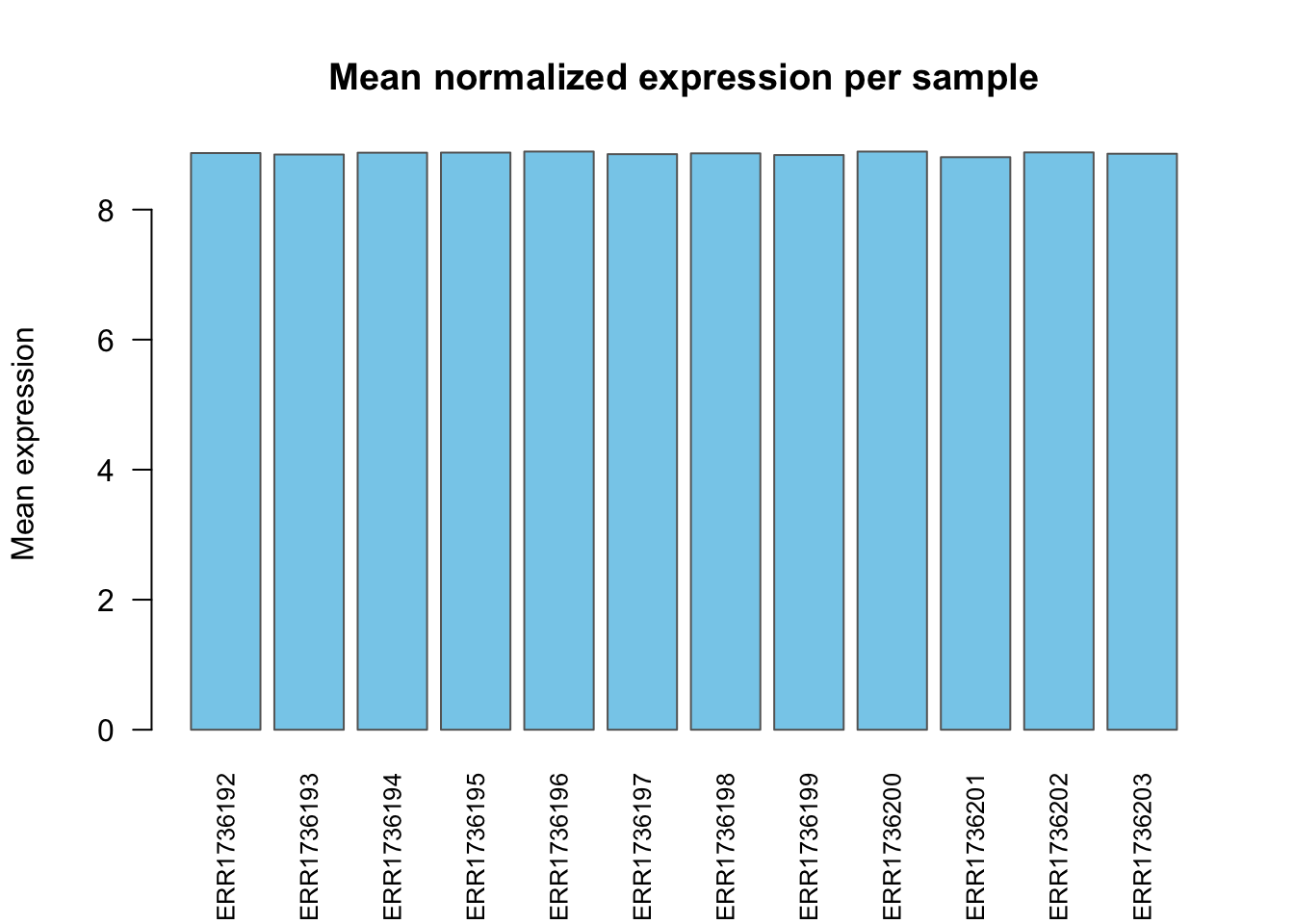

Exercise 2

Can you color the samples by their conditions?

Tip

cols <- ifelse(data$anno$compound == "sucrose", "tomato", "steelblue")
barplot(sample_means, las = 2, col = cols,
        main = "Mean expression per sample",
        ylab = "Mean expression", border = "gray40", cex.names = 0.8)
legend("topright", legend = c("none", "sucrose"),
       fill = c("steelblue", "tomato"), bty = "n")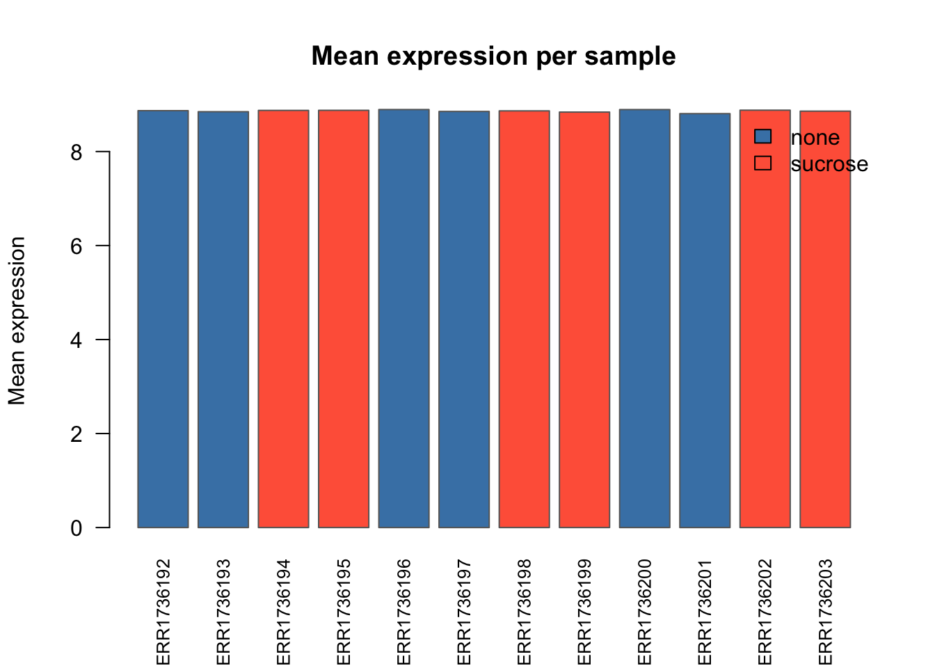

Volcano plot of results

head(data$diff)

      Gene_ID    Gene_name sucrose_24h_pval sucrose_24h_lfc sucrose_3h_pval
10  AT1G01090 PDH-E1 ALPHA        0.5905386             1.1       0.9983381
11  AT1G01100        RPP1A        0.5688959             1.1       0.9983381
33  AT1G01300         APF2        0.5650828             1.1       0.9983381
36  AT1G01320                     0.7427942             0.0       0.9983381
69  AT1G01620       PIP1-3        0.8840503             0.0       0.9983381
105 AT1G01960         BIG3        0.8171195             0.0       0.9983381
    sucrose_3h_lfc
10             0.0
11            -1.1
33             0.0
36             1.1
69            -1.1
105            0.0

Expression value distribution

hist(unlist(data$counts),
     breaks = 40, col = "lightgray", border = "gray40",
     main = "Distribution of normalized expression values",
     xlab = "Expression", ylab = "Frequency")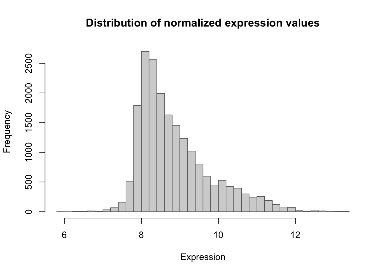

Exerise 3

Can you add density curve for smoothness?

Tip

hist(unlist(data$counts), breaks = 40, col = "lightgray", border = "gray40",
     freq = FALSE, main = "Expression value distribution", xlab = "Expression")
lines(density(unlist(data$counts)), col = "tomato", lwd = 2)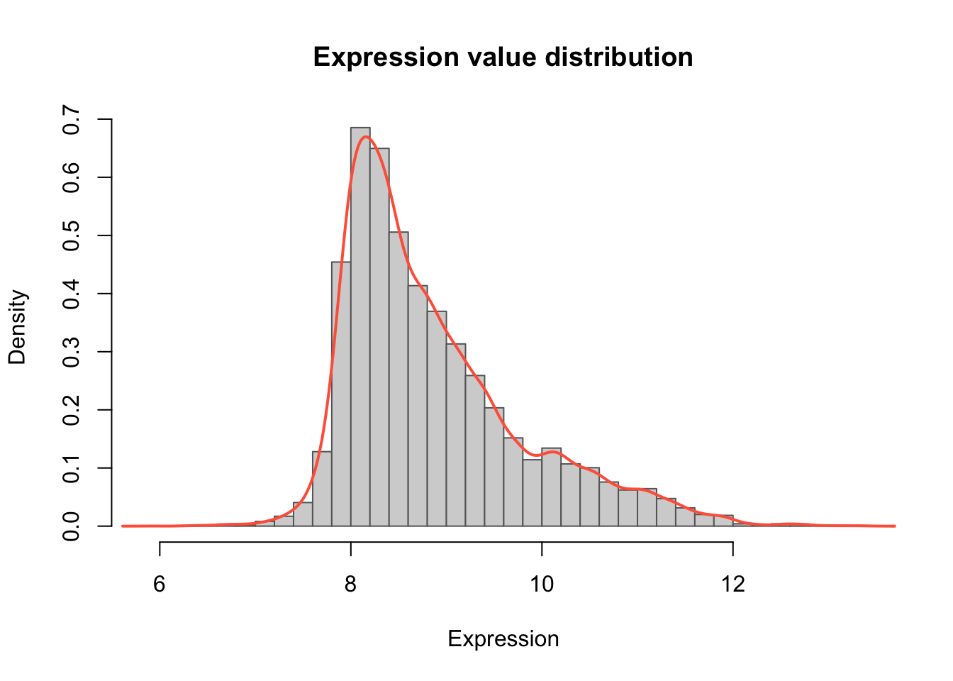

Volcano plot of differential results

Sucrose 24h

# Identify significant genes
sig_24h <- data$diff$sucrose_24h_pval < 0.05 & abs(data$diff$sucrose_24h_lfc) > 1

# Volcano plot
plot(data$diff$sucrose_24h_lfc,
     -log10(data$diff$sucrose_24h_pval),
     pch = 16, cex = 0.6,
     col = ifelse(sig_24h, "tomato", "gray70"),
     main = "Volcano Plot — Sucrose 24h",
     xlab = "log2 Fold Change",
     ylab = "-log10(p-value)")

# Add significance thresholds
abline(v = c(-1, 1), col = "red", lty = 2)
abline(h = -log10(0.05), col = "blue", lty = 2)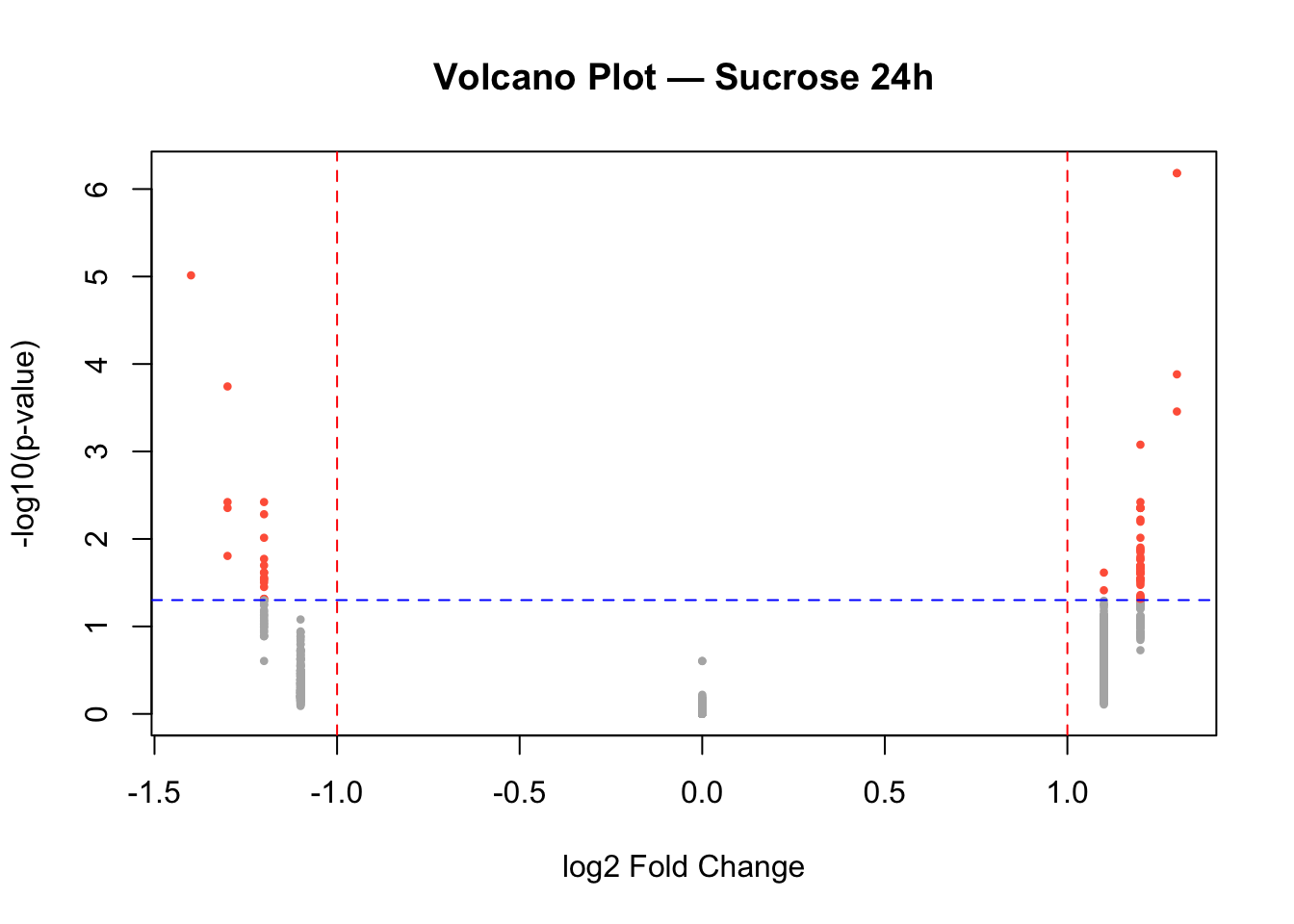

Sucrose 3h

# Identify significant genes
sig_3h <- data$diff$sucrose_3h_pval < 0.05 & abs(data$diff$sucrose_3h_lfc) > 1

# Volcano plot
plot(data$diff$sucrose_3h_lfc,
     -log10(data$diff$sucrose_3h_pval),
     pch = 16, cex = 0.6,
     col = ifelse(sig_3h, "tomato", "gray70"),
     main = "Volcano Plot — Sucrose 3h",
     xlab = "log2 Fold Change",
     ylab = "-log10(p-value)")

# Add significance thresholds
abline(v = c(-1, 1), col = "red", lty = 2)
abline(h = -log10(0.05), col = "blue", lty = 2)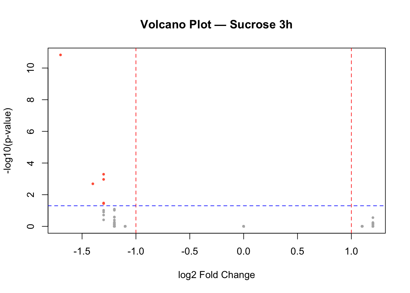

Exercise 4

Can you display both the plots together?

Tip

par(mfrow = c(1, 2))  # 1 row, 2 columns

# Volcano 24h
sig_24h <- data$diff$sucrose_24h_pval < 0.05 & abs(data$diff$sucrose_24h_lfc) > 1
plot(data$diff$sucrose_24h_lfc,
     -log10(data$diff$sucrose_24h_pval),
     pch = 16, cex = 0.6,
     col = ifelse(sig_24h, "tomato", "gray70"),
     main = "Volcano — Sucrose 24h",
     xlab = "log2 Fold Change", ylab = "-log10(p-value)")
abline(v = c(-1, 1), col = "red", lty = 2)
abline(h = -log10(0.05), col = "blue", lty = 2)

# Volcano 3h
sig_3h <- data$diff$sucrose_3h_pval < 0.05 & abs(data$diff$sucrose_3h_lfc) > 1
plot(data$diff$sucrose_3h_lfc,
     -log10(data$diff$sucrose_3h_pval),
     pch = 16, cex = 0.6,
     col = ifelse(sig_3h, "tomato", "gray70"),
     main = "Volcano — Sucrose 3h",
     xlab = "log2 Fold Change", ylab = "-log10(p-value)")
abline(v = c(-1, 1), col = "red", lty = 2)
abline(h = -log10(0.05), col = "blue", lty = 2)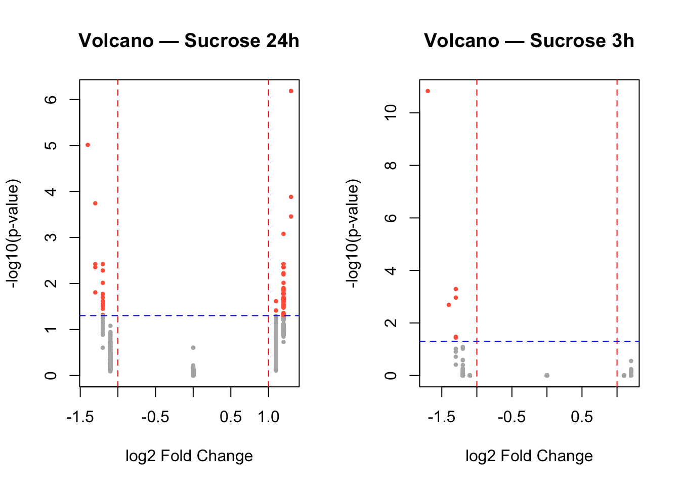

par(mfrow = c(1, 1))  # Reset layout

Session information

Tip

sessionInfo()

R version 4.5.1 (2025-06-13)
Platform: aarch64-apple-darwin20
Running under: macOS Tahoe 26.0.1

Matrix products: default
BLAS:   /Library/Frameworks/R.framework/Versions/4.5-arm64/Resources/lib/libRblas.0.dylib 
LAPACK: /Library/Frameworks/R.framework/Versions/4.5-arm64/Resources/lib/libRlapack.dylib;  LAPACK version 3.12.1

locale:
[1] en_US.UTF-8/en_US.UTF-8/en_US.UTF-8/C/en_US.UTF-8/en_US.UTF-8

time zone: Europe/Zurich
tzcode source: internal

attached base packages:
[1] stats     graphics  grDevices datasets  utils     methods   base     

loaded via a namespace (and not attached):
 [1] htmlwidgets_1.6.4   BiocManager_1.30.26 compiler_4.5.1     
 [4] fastmap_1.2.0       cli_3.6.5           htmltools_0.5.8.1  
 [7] tools_4.5.1         yaml_2.3.10         rmarkdown_2.30     
[10] knitr_1.50          jsonlite_2.0.0      xfun_0.53          
[13] digest_0.6.37       rlang_1.1.6         renv_1.1.5         
[16] evaluate_1.0.5